I’ve just finished R for Data Science by Hadley Wickham and just started Text mining With R by Julia Silge. So I figured it’s about time i do some data analysis to apply the skills I learned. I decided to do sentiment analysis after reading this post by Julia Silge.
After skimming through some interesting datasets on the internet, i decided to use ’A Million Headlines` dataset which can be found on Kaggle. It’s a dataset of news headlines published over a period of 14 years from 2003 to 2017 taken from Australian news source ABC(Australian Broadcasting Group).
First, let’s import all the packages needed:
library(tidyverse)
library(here)
library(tidytext)
library(viridis)
library(widyr)
library(ggraph)
library(igraph)
library(scales)
library(knitr)
library(wordcloud)
library(reshape2)
Now let’s import the data
# import data
news <- as.tibble(read_csv(here("abcnews-date-text.csv")))
news
## # A tibble: 1,103,665 x 2
## publish_date headline_text
## <dbl> <chr>
## 1 20030219 aba decides against community broadcasting licence
## 2 20030219 act fire witnesses must be aware of defamation
## 3 20030219 a g calls for infrastructure protection summit
## 4 20030219 air nz staff in aust strike for pay rise
## 5 20030219 air nz strike to affect australian travellers
## 6 20030219 ambitious olsson wins triple jump
## 7 20030219 antic delighted with record breaking barca
## 8 20030219 aussie qualifier stosur wastes four memphis match
## 9 20030219 aust addresses un security council over iraq
## 10 20030219 australia is locked into war timetable opp
## # ... with 1,103,655 more rowsTerm Frequency
One of the common task in text mining is to look at word frequencies. Let’s analyze word frequencies in all of the headlines
news <- news %>%
      # create year column
      mutate(year = substr(publish_date,
                start = 1, stop = 4),
                linenumber = row_number())

news
## # A tibble: 1,103,665 x 4
## publish_date headline_text year linenumber
## <dbl> <chr> <chr> <int>
## 1 20030219 aba decides against community broadcasti… 2003 1
## 2 20030219 act fire witnesses must be aware of defa… 2003 2
## 3 20030219 a g calls for infrastructure protection … 2003 3
## 4 20030219 air nz staff in aust strike for pay rise 2003 4
## 5 20030219 air nz strike to affect australian trave… 2003 5
## 6 20030219 ambitious olsson wins triple jump 2003 6
## 7 20030219 antic delighted with record breaking bar… 2003 7
## 8 20030219 aussie qualifier stosur wastes four memp… 2003 8
## 9 20030219 aust addresses un security council over … 2003 9
## 10 20030219 australia is locked into war timetable o… 2003 10
## # ... with 1,103,655 more rowswe can use unnest_tokens to separate each line into words. The default tokenizing is for words, but other options include characters, sentences, lines, paragraphs, or separation around regex pattern.
tidy_news <- news %>%
        unnest_tokens(word, headline_text)

tidy_news
## # A tibble: 7,070,525 x 4
## publish_date year linenumber word
## <dbl> <chr> <int> <chr>
## 1 20030219 2003 1 aba
## 2 20030219 2003 1 decides
## 3 20030219 2003 1 against
## 4 20030219 2003 1 community
## 5 20030219 2003 1 broadcasting
## 6 20030219 2003 1 licence
## 7 20030219 2003 2 act
## 8 20030219 2003 2 fire
## 9 20030219 2003 2 witnesses
## 10 20030219 2003 2 must
## # ... with 7,070,515 more rowsNow we can manipulate the data and do term frequency analysis. First, let’s remove stop words which can be obtain from dataset stop_words with the function anti_join. Stop words are words which do not contain important significance. We filter out stop words as it could affect our analysis.
# remove stopwords

data("stop_words")
tidy_news <- tidy_news %>%
        anti_join(stop_words)
Let’s see the most frequent words use in the news headlines since 2003:
# most common words
tidy_news %>%
    count(word, sort = TRUE) %>%
    head(20) %>%
    mutate(word = reorder(word, n)) %>%
    ggplot(aes(word, n)) +
    geom_bar(stat = "identity") +
    coord_flip() +
    ylab("Number of occurences") +
    xlab("Word")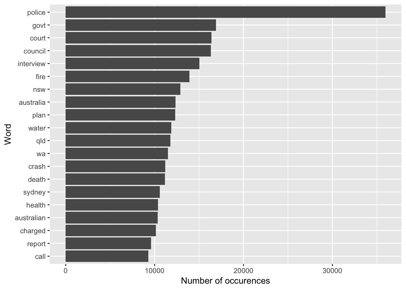
We can see here most of the headlines contain the words, “police”, “court”, “council”.
Network of Words
Let’s count the words that occur together in the headlines from 2017. Using pairwise_count function from widyr package, we can count highest co-occurances pair of words.
headlines_2017 <- tidy_news %>%
    filter(year == "2017") %>%
    pairwise_count(word, linenumber, sort = TRUE)

headlines_2017
## # A tibble: 1,004,826 x 3
## item1 item2 n
## <chr> <chr> <dbl>
## 1 trump donald 612
## 2 donald trump 612
## 3 korea north 301
## 4 north korea 301
## 5 marriage sex 285
## 6 sex marriage 285
## 7 turnbull malcolm 197
## 8 malcolm turnbull 197
## 9 election wa 149
## 10 wa election 149
## # ... with 1,004,816 more rowsDonald trump is the highest occurences pair of words in 2017 followed by North Korea which unsurprising as the feud between them bring fear about nuclear war around the world. Also in 2017, Australia vote in favour of legalising same sex marriage which is big news across the country. Hence explains why sex marriage is just below Donald Trump and North Korea in frequency of co-occurences pair of words in 2017 headlines.
Let’s plot the network of words occurences:
#pairwise count
word_pairs <- tidy_news %>%
  group_by(word) %>%
  filter(n() > 5) %>%
  ungroup() %>%
  pairwise_count(item=word,
                 linenumber, sort = TRUE,
                 upper = FALSE) %>%
  filter(n > 10)

#create plot
word_pairs %>%
  top_n(100) %>%
        graph_from_data_frame() %>%
        ggraph(layout = "fr") +
        geom_edge_link(aes(edge_alpha = n,
                           edge_width = n)) +
        geom_node_point(color = "darkslategray4",
                        size = 5) +
        geom_node_text(aes(label = name),
                       vjust = 1.8) +
        ggtitle(expression(paste(
                  "Word Network in ABC Headlines From
                  2003-2017"))) +
        theme_void()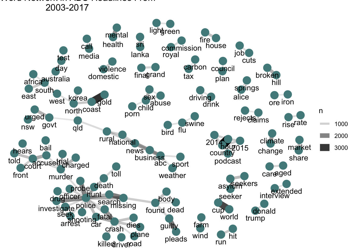
Next, we’ll look into sentiment analysis of these words so we can understand what type of sentiment have been used in most of these headlines.
Sentiment Analysis
Now let’s investigate sentiment analysis. When we reads a text, we use our understanding of the emotional intent of words to infer wheter a section of words is positive or negative and also categorized it into emotion like anger or joy. Let’s use bing lexicon from sentiments dataset to categorized our words into positive or negative sentiment.
# create dataframe of words from bing lexicon
library(tidyr)
bing <- sentiments %>%
        filter(lexicon == "bing") %>%
        select(-score)

bing
## # A tibble: 6,788 x 3
## word sentiment lexicon
## <chr> <chr> <chr>
## 1 2-faced negative bing
## 2 2-faces negative bing
## 3 a+ positive bing
## 4 abnormal negative bing
## 5 abolish negative bing
## 6 abominable negative bing
## 7 abominably negative bing
## 8 abominate negative bing
## 9 abomination negative bing
## 10 abort negative bing
## # ... with 6,778 more rowsUsing inner_join function, we can categorized the words into positive or negative by joining bing dataset.
# classified words into positive
## or negative based on bing lexicon
news_sentiment <- tidy_news %>%
        inner_join(bing) %>%
        count(year,sentiment) %>%
        spread(sentiment, n, fill = 0) %>%
        mutate(sentiment = positive - negative)

news_sentiment
## # A tibble: 15 x 4
## year negative positive sentiment
## <chr> <dbl> <dbl> <dbl>
## 1 2003 26303 12604 -13699
## 2 2004 31093 14291 -16802
## 3 2005 31705 13522 -18183
## 4 2006 28471 12123 -16348
## 5 2007 32875 13454 -19421
## 6 2008 34001 14123 -19878
## 7 2009 32679 13069 -19610
## 8 2010 31273 12589 -18684
## 9 2011 30169 11997 -18172
## 10 2012 30152 13555 -16597
## 11 2013 31884 14523 -17361
## 12 2014 28363 14290 -14073
## 13 2015 30389 14673 -15716
## 14 2016 24249 11487 -12762
## 15 2017 19247 9208 -10039Most common positive and negative words
Now that we have data frame of positive and negative sentiments, we can analyze which words is most common in the positive and negative category. We can filter out NA sentiment or neutral sentiment.
word_count <- tidy_news %>%
  left_join(get_sentiments("bing"), by = "word") %>%
  filter(!is.na(sentiment)) %>%
  count(word, sentiment, sort = TRUE) %>%
  ungroup()

top_sentiments_bing <- word_count %>%
          filter(word != "wins") %>%
          group_by(sentiment) %>%
          top_n(5, n) %>%
          mutate(num = ifelse(sentiment == "negative",
                              -n, n)) %>%
          mutate(word = reorder(word, num)) %>%
          ungroup()

top_sentiments_bing
## # A tibble: 10 x 4
## word sentiment n num
## <chr> <chr> <int> <int>
## 1 crash negative 11208 -11208
## 2 death negative 11173 -11173
## 3 murder negative 9217 -9217
## 4 win positive 8315 8315
## 5 killed negative 8129 -8129
## 6 attack negative 7166 -7166
## 7 boost positive 6997 6997
## 8 gold positive 6211 6211
## 9 top positive 5687 5687
## 10 support positive 5399 5399Let’s see top 5 words from positive and negative sentiment.
ggplot(top_sentiments_bing, aes(reorder(word, num), num,
                                fill = sentiment)) +
  geom_bar(stat = 'identity', alpha = 0.75) +
  scale_fill_manual(guide = F, values = c("black",
                                          "darkgreen")) +
  scale_y_continuous(breaks = pretty_breaks(7)) +
  labs(x = '', y = "Number of Occurrences",
       title = 'News Headlines Sentiments',
       subtitle = 'Most Common Positive and Negative Words') +
  theme_bw() +
  theme(axis.text.x = element_text(angle = 45, hjust = 1,
                                   size = 14, face = "bold"),
        panel.grid.minor = element_blank(),
        panel.grid.major.x = element_blank(),
        panel.grid.major.y = element_line(size = 1.1))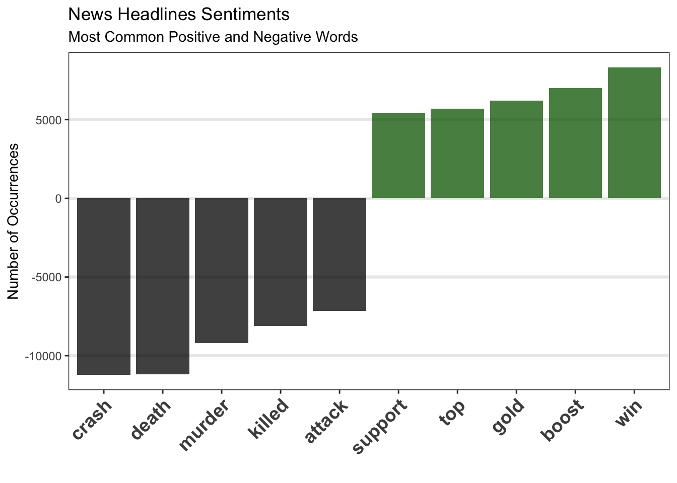
Word Cloud: Most Common Positive and Negative Words in News Headlines
library(wordcloud)   # to create wordcloud
library(reshape2)    # for acast() function

tidy_news %>%
  inner_join(bing) %>%
  count(word, sentiment, sort = TRUE) %>%
  acast(word ~ sentiment, value.var = "n", fill = 0) %>%
  comparison.cloud(colors = c("black", "darkgreen"),
                   title.size = 1.5)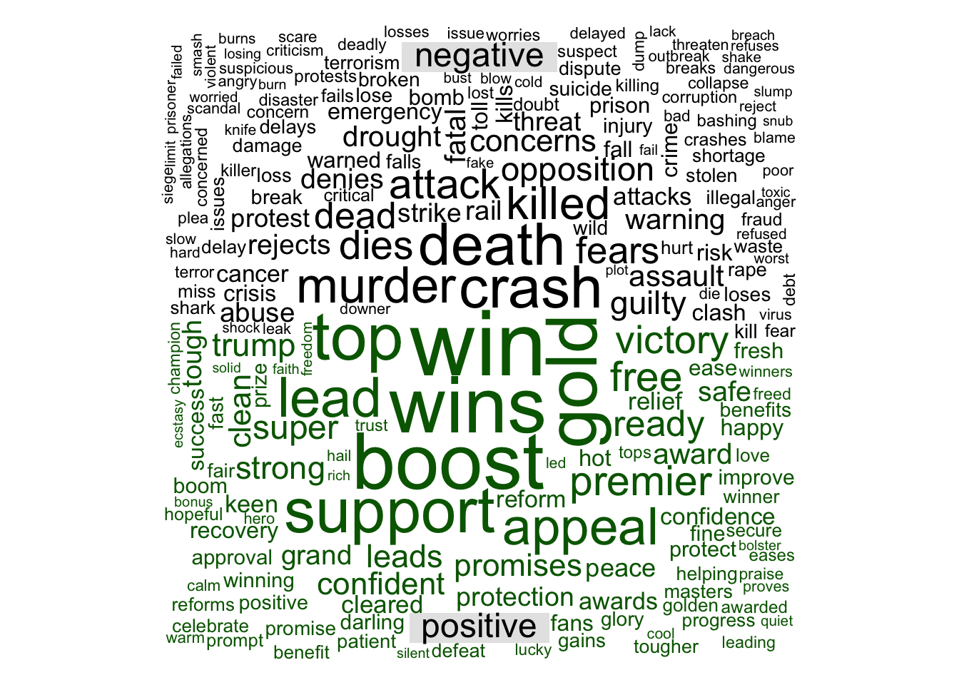
Proportions of Positive and Negative Words
Now let’s see the proportions of negative and positive words to entire data set. after filtering out words categorized as neutral, we calculate the frequency by first grouping them along sentiment then counting the rows for each of these groups. Finally, we can calculate the percentage by dividing the sum of all the rows in the data set.
sentiment_bing <- tidy_news %>%
        left_join(get_sentiments("bing"), by = "word") %>%
        filter(!is.na(sentiment)) %>%
        group_by(year, sentiment) %>%
        summarise(n = n()) %>%
        mutate(percent = n / sum(n)) %>%
        ungroup()

sentiment_bing
## # A tibble: 30 x 4
## year sentiment n percent
## <chr> <chr> <int> <dbl>
## 1 2003 negative 26303 0.676
## 2 2003 positive 12604 0.324
## 3 2004 negative 31093 0.685
## 4 2004 positive 14291 0.315
## 5 2005 negative 31705 0.701
## 6 2005 positive 13522 0.299
## 7 2006 negative 28471 0.701
## 8 2006 positive 12123 0.299
## 9 2007 negative 32875 0.710
## 10 2007 positive 13454 0.290
## # ... with 20 more rowssentiment_bing %>%
ggplot(aes(x = year, y = percent, color = sentiment,
group = sentiment)) +
geom_line(size = 1) +
geom_point(size = 3) +
scale_y_continuous(breaks = pretty_breaks(5),
labels = percent_format()) +
labs(x = "Album", y = "Emotion Words Count (as %)") +
scale_color_manual(values = c(positive = "darkgreen",
negative = "black")) +
ggtitle("Proportion of Positive and Negative Words",
subtitle = "Bing lexicon") +
theme_bw() +
theme(axis.text.x = element_text(angle = 45, hjust = 1,
size = 11, face = "bold"),
axis.title.x = element_blank(),
axis.text.y = element_text(size = 11, face = "bold"))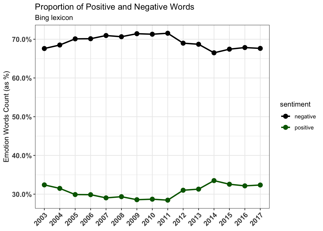
The proportion of negative sentiment words has been consistently much higher than proportion of positive sentiment words since 2003.
Let’s use NRC lexicon for sentiment analysis. NRC sentiments got list of sentiments way beyond positive and negative, it categorizes words into eight different emotion terms, Anger, Anticipation, Disgust, Fear, Joy, Sadness, Surprise, and Trust.
library(RColorBrewer)
cols <- colorRampPalette(brewer.pal(n = 8, name = "Set1"))(8)

cols
## [1] "#E41A1C" "#377EB8" "#4DAF4A" "#984EA3" "#FF7F00" "#FFFF33" "#A65628"
## [8] "#F781BF"Now, let’s plot the distribution of emotion terms on boxplot:
cols <- c("anger" = "#E41A1C", "sadness" = "#377EB8",
          "disgust" = "#4DAF4A", "fear" = "#984EA3",
          "surprise" = "#FF7F00", "joy" = "#FFFF33",
          "anticipation" = "#A65628", "trust" = "#F781BF")

news_nrc <- tidy_news %>%
  left_join(get_sentiments("nrc"), by = "word") %>%
  filter(!(sentiment == "negative" |
           sentiment == "positive")) %>%
  mutate(sentiment = as.factor(sentiment)) %>%
  group_by(index = linenumber %/% 100,
           sentiment) %>%
  summarize(n = n()) %>%
  mutate(percent = n / sum(n)) %>%
  select(-n) %>%
  ungroup()

library(hrbrthemes)

news_nrc %>%
  ggplot() +
  geom_boxplot(aes(x = reorder(sentiment, percent),
                   y = percent, fill = sentiment)) +
  scale_y_continuous(breaks = pretty_breaks(5),
                     labels = percent_format()) +
  scale_fill_manual(values = cols) +
  ggtitle("Distribution of Emotion Terms") +
  labs(x = "Emotion Term", y = "Percentage") +
  theme_bw() +
  theme(legend.position = "none",
        axis.text.x = element_text(size = 11,
                                   face = "bold"),
        axis.text.y = element_text(size = 11,
                                   face = "bold"))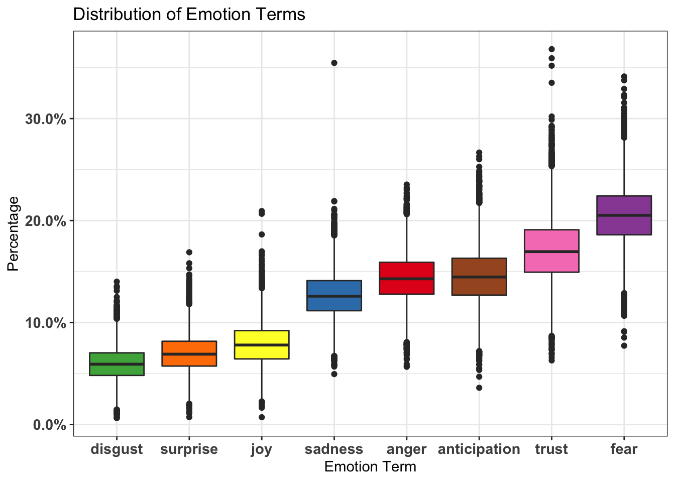
Fear has highest percentage in the distribution. Next, we can see how the sentiment emotions of headlines change over time by creating bump chart that plots different sentiment groups
news_nrc2 <- tidy_news %>%
  left_join(get_sentiments("nrc"), by = "word") %>%
  filter(!(sentiment == "negative" |
             sentiment == "positive")) %>%
  mutate(sentiment = as.factor(sentiment)) %>%
  group_by(year, sentiment) %>%
  summarize(n = n()) %>%
  mutate(percent = n / sum(n)) %>%
  select(-n) %>%
  ungroup()


news_nrc2 %>%
  group_by(year) %>%
  ggplot(aes(year, percent, color = sentiment,
             group = sentiment)) +
  geom_line(size = 1) +
  geom_point(size = 3.5) +
  scale_y_continuous(breaks = pretty_breaks(5),
                     labels = percent_format()) +
  xlab("Year") + ylab("Proportion of Emotion Words") +
  ggtitle("News Headlines Sentiments Across Years",
          subtitle = "From 2003-2017") +
  theme_bw() +
  theme(axis.text.x = element_text(angle = 45,
                                   hjust = 1, size = 11,
                                   face = "bold"),
        axis.title.x = element_blank(),
        axis.text.y = element_text(size = 11,
                                   face = "bold")) +
  scale_color_brewer(palette = "Set1")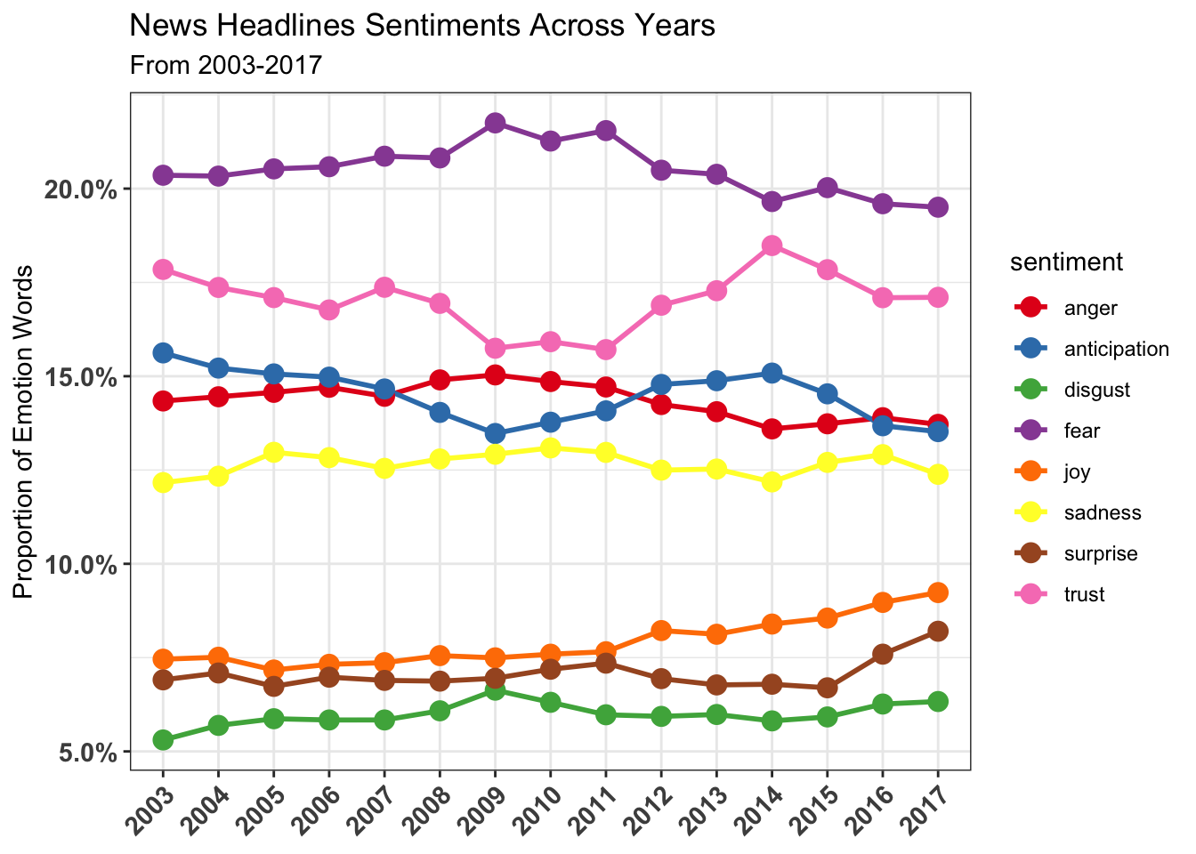
We can see that the sentiment changes over time is quite consistent, with fear sentiment already at high level in 2003.
Let’s see what are the most words used that are associated with fear:
nrc_fear <- get_sentiments("nrc") %>%
  filter(sentiment == "fear")

tidy_news %>%
  inner_join(nrc_fear) %>%
  count(word, sort = TRUE)
## # A tibble: 1,300 x 2
## word n
## <chr> <int>
## 1 police 35985
## 2 court 16380
## 3 fire 13910
## 4 crash 11208
## 5 death 11173
## 6 murder 9217
## 7 hospital 8815
## 8 accused 8094
## 9 government 7905
## 10 missing 7582
## # ... with 1,290 more rows“police”, “fire”, “crash” are few of words associated with fear with the word “court” being the highest count.
Comparing how sentiments differ across the sentiment libraries
There’s three options for sentiment lexicons, let’s see how the three sentiment lexicon differ when used for these headlines.
First, let’s see how many positive and negative words each lexicon categorized.
Bing
get_sentiments("bing") %>%
  count(sentiment)
## # A tibble: 2 x 2
## sentiment n
## <chr> <int>
## 1 negative 4782
## 2 positive 2006NRC
get_sentiments("nrc") %>%
  count(sentiment)
## # A tibble: 10 x 2
## sentiment n
## <chr> <int>
## 1 anger 1247
## 2 anticipation 839
## 3 disgust 1058
## 4 fear 1476
## 5 joy 689
## 6 negative 3324
## 7 positive 2312
## 8 sadness 1191
## 9 surprise 534
## 10 trust 1231- Bing: there are 4782 words that can be categorized as negative, and 2006 positive.
- NRC : there are 3324 words that are categorized as negative, and 2312 positive.
The proportion of negative words in Bing lexicon is much higher than proportion of negative words in NRC lexicon.
Let’s count how many words in our text are categorized for each sentiment:
# Bing lexicon
tidy_news %>%
  left_join(get_sentiments("bing"), by = "word") %>%
  group_by(sentiment) %>%
  summarize(sum = n())
## # A tibble: 3 x 2
## sentiment sum
## <chr> <int>
## 1 negative 442853
## 2 positive 195508
## 3 <NA> 4706155# nrc lexicon
tidy_news %>%
left_join(get_sentiments("nrc"), by = "word") %>%
group_by(sentiment) %>%
summarize(sum = n())## # A tibble: 11 x 2
## sentiment sum
## <chr> <int>
## 1 anger 306856
## 2 anticipation 309873
## 3 disgust 127805
## 4 fear 438814
## 5 joy 168191
## 6 negative 555330
## 7 positive 518200
## 8 sadness 270419
## 9 surprise 150105
## 10 trust 363695
## 11 <NA> 4027259- For Bing: 193, 549 words are categorized as negative and 193,549 words are positive.
- For NRC: 549191 words are categorized as negative and 512,498 positive
In summary, NRC lexicon managed to categorized the words much more than Bing lexicon did.
Let’s see how AFINN lexicon categorized the words now, as it’s the only lexicon we haven’t touched yet in the tidytext package! The AFINN lexicon gives a score from -5 (for negative sentiment) to +5 (positive sentiment).
AFINN
headlines_afinn <- tidy_news %>%
  left_join(get_sentiments("afinn"), by = "word") %>%
  filter(!grepl('[0-9]', word))

# count NA category
headlines_afinn %>%
    summarize(NAs= sum(is.na(score)))
## # A tibble: 1 x 1
## NAs
## <int>
## 1 4584704headlines_afinn %>%
select(score) %>%
mutate(sentiment = if_else(score > 0,
"positive", "negative",
"NA")) %>%
group_by(sentiment) %>%
summarize(sum = n())## # A tibble: 3 x 2
## sentiment sum
## <chr> <int>
## 1 NA 4584704
## 2 negative 469070
## 3 positive 204720There are 4,532,575 words out of 5, 199, 782 words that was not categorized by AFINN. Let’s visualize scoring ability of each lexicon.
afinn_scores <- headlines_afinn %>%
  replace_na(replace = list(score = 0)) %>%
  group_by(index = linenumber %/% 10000) %>%
  summarize(sentiment = sum(score)) %>%
  mutate(lexicon = "AFINN")

# combine the Bing and NRC lexicons into one data frame:

bing_nrc_scores <- bind_rows(
  tidy_news %>%
    inner_join(get_sentiments("bing")) %>%
    mutate(lexicon = "Bing"),
  tidy_news %>%
    inner_join(get_sentiments("nrc") %>%
                 filter(sentiment %in% c("positive",
                                         "negative"))) %>%
    mutate(lexicon = "NRC")) %>%
  # from here we count the sentiments,
  ## then spread on positive/negative, then create the score:
  count(lexicon, index = linenumber %/% 10000,
        sentiment) %>%
  spread(sentiment, n, fill = 0) %>%
  mutate(lexicon = as.factor(lexicon),
         sentiment = positive - negative)

# combine all lexicons into one data frame
all_lexicons <- bind_rows(afinn_scores, bing_nrc_scores)
lexicon_cols <- c("AFINN" = "#E41A1C",
                  "NRC" = "#377EB8", "Bing" = "#4DAF4A")

all_lexicons
## # A tibble: 333 x 5
## index sentiment lexicon negative positive
## <dbl> <dbl> <chr> <dbl> <dbl>
## 1 0 -5364 AFINN NA NA
## 2 1 -3761 AFINN NA NA
## 3 2 -3952 AFINN NA NA
## 4 3 -4294 AFINN NA NA
## 5 4 -4481 AFINN NA NA
## 6 5 -4077 AFINN NA NA
## 7 6 -4979 AFINN NA NA
## 8 7 -4659 AFINN NA NA
## 9 8 -5018 AFINN NA NA
## 10 9 -5087 AFINN NA NA
## # ... with 323 more rowsall_lexicons %>%
ggplot(aes(index, sentiment, fill = lexicon)) +
geom_col() +
facet_wrap(~lexicon, ncol = 1, scales = "free_y") +
scale_fill_manual(values = lexicon_cols) +
ggtitle("Comparison of Sentiments") +
labs(x = "Index of All Headlines From 2003-2017" ,
y = "Sentiment Score") +
theme_bw() +
theme(axis.text.x = element_blank())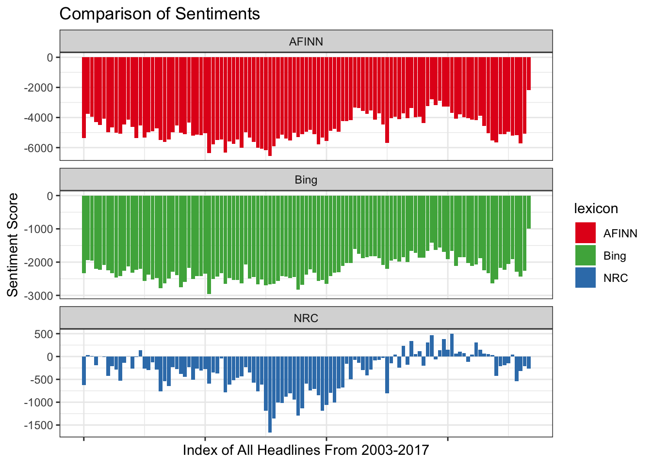
We can see that AFINN and Bing lexicon sentiment across the years have been negative, there’s really no positive sentiment at all! But we can see in the latest index the negative score is really small, is the trend changing? we need more data to confirm that.
Generally, across all lexicon, the sentiment of the headlines has all been negative.
Summary
We can see from the analysis that negative sentiment has been dominating media headlines in Australia since 2013 with fear being the dominating theme emotion. Most of these negative sentiment came from reporting of crime, automobile crash etc.These types of headlines are the most appealing to readers, hence why their term frequencies are high. However, the 3 lexicons we used in this analysis failed to categorized so many words in all the headlines. To be exact, there are 4,652,959, 3,982,132, and 4,532,575 words that are not categorized by Bing, NRC, and AFINN lexicon consecutively.
It is important to note that lexicons in the tidytext package are not the be all and end all for text/sentiment analysis. One can even create their own lexicons through crowd-sourcing (such as Amazon Mechanical-Turk, which is how some of the lexicons shown here were created), from utilizing word lists accrued by your own company throughout the years dealing with customer/employee feedback, etc. It would be interesting to compare this datasets with headlines from another country. For example, we can compare the most focused term used by headlines in different country using the tf-idf statistic.